Path planner for deployment
Motivation and rationale
During the phase before purse seine deployment the purse seine master (“the purser”) needs to acquire and maintain a situational awareness. This is a key success factor in purse seining. Elements of the situational awareness include a comprehension of the main process components in play. A firm comprehension increases the rate of success and the diminishes the probability of disastrous failure due to malpractice. Mastery of purse seining is often correlated with experience. Regardless of the level of experience, there is a fair amount of burden placed on the purser. For this reason, a useful aid would be a tool that could both ease the burden and help acquire the necessary situational awareness. Let us for now denote this tool as an on-board decision support system (ODSS) [28].
Modern purse seiners are equipped with sophisticated instruments, which help the captain in executing their job. The wheel house has many monitors with diverse and scattered information, from which some are very important during the pre-deployment phase. A proficient purser possesses both perceptive and predictive abilities. This means that based on the available sensory information about the processes in play, the purser is capable of predicting ahead in time a plausible outcome based on a series of actions. These actions are typically, i) to purposefully maneuver the vessel, and ii) to determine an appropriate time point for purse deployment in such a way that the fish is caught as intended.
The procedure has several similarities with a typical optimal control problem, which help justify our chosen plan of attack in developing a tool in form of an ODSS. This is because, in many aspects, the purser is a model predictive controller with the objective to optimally execute a purse seine deployment. From the above description it is clear that the following features are important:
Ability to make use of available sensory information;
Comprehension of the main process components;
Possess predictive capabilities;
Devising a set of purposeful actions;
Fulfill a well-defined purpose, which has a specific objective.
Coincidentally, these features also signify successful building blocks in an optimal control problem [6]. Our rationale for choosing mathematical optimization as the problem solving approach is mainly due to the likeness of features, but it is not the sole reason. One other important justification is the flexibility in problem formulation and, in effect, the possible solution space. With this, we mean that there may be user-specific preferences, which have implications for the decision support presented to the user. Moreover, the flexibility in problem description also facilitates adaptations and improvements with little additional effort. This effort may include better model descriptions based on new data or other tweaks to the mathematical modeling.
Problem statement of the purse seine path planner
The goal is to create an ODSS for purse seine deployment. We proceed by establishing central building blocks for the optimal control problem formulation. Specifically, we need to describe in detail the features as listed above. We pose the formulation as a so-called path planning problem. A solution to this problem contains the following:
A suggested planar path for the fishing vessel to follow;
An indicated point in time and space for initiation of purse deployment;
Auxiliary information about the involved actors, which helps situational awareness.
Typically, such solutions should be presented to the purser in an informative manner, such as a graphical visualization including a map plot 1 . The arrows in Fig. 4 indicate information flow and interactions between important elements of the presented decision support. Instruments are capable of acquiring relevant environmental data together with vessel-specific measurements in real time. We assume that there exists a machine-to-machine application programming interface that are capable of sharing this information, for instance “Ratatosk” [25] 2 . Herein, we focus on the mathematical modeling of the Online path planner indicated in Fig. 4.
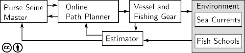
Fig. 4 Main elements in a purse seine deployment process.
From a path planning perspective, the relevant phases of a purse seine deployment are the pre-deployment positioning and the purse deployment circling [5]. Questions in need of answers are, where is the school, where will it go, what is the current, how should we maneuver the vessel, where and when should we initiate deployment, will the net sink quick and deep enough. The path planner problem is stated in Problem 8.
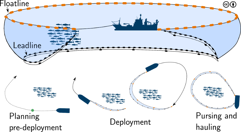
Fig. 5 Purse Seine.
Problem 8 (Purse seine path planning)
Find an ideal vessel trajectory to surround the targeted fish school, subject to:
Purse planner formulation
Our hypothesis is that an optimization-based algorithm can conceive a sound course of actions based on predictive capabilities. The conception takes form by mathematically describing principal components of the system to a sufficient fidelity. Hence, we formalize Problem 8 by utilizing common modeling techniques such as first principles, datasets and engineering cleverness. We should arrive at an optimal control problem formulation, which can be efficiently solved using numerical techniques for nonlinear programming problems [4, 6, 7]. The principal components in need of scrutiny are:
Fishing vessel;
Fish school;
Leadline sinking response;
Environment’s impact on above components;
Criteria for ideal vessel trajectory and deployment initiation.
An important aspect of the formulation is that of timing with respect to the leadline sinking in relation to fish school and vessel trajectories. We identify four time points that signify key events of the purse deployment process, namely:
Deployment initiation at deployment point \(p_d\), at time point \(t_d\);
Leadline enters waters at collision point \(p_c\), at time point \(t_s\);
Fish is surrounded, at time point \(t_{pd}\).
Fish arrives at collision point \(p_c\), at time point \(t_c\);
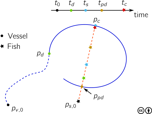
Fig. 6 Overview of key time points of the deployment process.
At these time points, the vessel and the fish school are located at various positions in relation to each other and is indicated in Fig. 6. The main objective of the planner is to determine the deployment time while fulfilling various criteria for a successful deployment. In the following sections, we will describe the principal components and combine them with additional descriptions to solve the timing and trajectory planning problem. Some descriptions are located in Appendix.
Notation
We denote an inertial reference frame with axes \(x\), \(y\), and \(z\) pointing north, east, down as \(\{\text{NED}\}\).
Define a limited time horizon \(\mathbb{T} := \{t \in \mathbb{R} : t_0 \leq t \leq t_f\}\), where \(t_f>t_0\geq 0\).
The partial derivative of a function \(f(x,y)\) is written with a superscript \(\frac{d f(x)}{dx} = f^x(x,y)\).
If the argument is time, we use the common dot notation, i.e. \(\frac{dx(t)}{dt} = \dat x(t)\).
The orientation space is defined by \(\mathbb{S} \in [-\pi,\pi)\).
\(I_n\) is the \(n\times n\) identity matrix.
\(1_{n\times m}\) is an \(n\text{-by-}m\) matrix of ones.
\(0_{n\times m}\) is an \(n\text{-by-}m\) matrix of zeros.
A block diagonal matrix of other matrices \(X_{i\in \mathbb{I}_{>,s}} \in \mathbb{R}^{m_i\times n_i}\) is defined as \(\bdiag_{i \in \mathbb{I}_{>,s}}(X_i) := \bigoplus_{i \in \mathbb{I}_{>,s}} X_i\), where \(\oplus\) is the direct sum.
The symbol \(\otimes\) is the Kronecker product.
The vertically stacked matrix of other matrices \(X_{i \in \mathbb{I}_{>,s}} \in \mathbb{R}^{m_i \times n}\) is denoted \(\col_{i \in \mathbb{I}_{>,s}}(X_i) := \bdiag_{i\in \mathbb{I}_{>,s}}(X_i) \cdot (1_{s \times 1} \otimes I_n)\).
The horizontally stacked matrix of other matrices \(X_{i \in \mathbb{I}_{>,s}} \in \mathbb{R}^{m \times n_i}\) is denoted \(\row_{i \in \mathbb{I}_{>,s}}(X_i) := \col_{i\in \mathbb{I}_{>,s}}(X_i^T)^T\).
Sea current and surface current water frame
Suppose the sea current is given by \(v_c(p,t): \mathbb{R}^3 \times \mathbb{R} \to \mathbb{R}^3\), where \(p\) is a position in \(\{\text{NED}\}\). We assume that the current is slowly-varying and can be approximated in a region of interest by a vertical vector field, which is independent of planar position. The sea current is thus assumed constant in each depth layer for a limited time horizon, and is approximated by \(w_c(p_z; t_0) \approx v_c(p,t)\, \forall t \in \mathbb{T}\).
We will make use of a reference frame that moves with the surface current, denoted water frame, \(\{\text{WF}\}\), with axes aligned with \(\{\text{NED}\}\). The constant planar surface current can be written in polar form as
where the origin of the water frame in \(\{\text{NED}\}\) is written as an initial value problem
Notice that the initial value of the water frame is always set to the origin.
Fishing vessel
We need a dynamic model that has enough fidelity to allow us to devise maneuverable paths. The fishing vessel is described as a planar kinematic vehicle under the influence of sea current. The planar position of the vessel on the \(xy\text{-plane}\) of \(\{\text{NED}\}\) is \(p_v(t) \in \mathbb{R}^2\). Define \(U_v>0\) as the speed in water. Let \(\psi_v(t) \in \mathbb{R}\) be the heading of the vessel, that is, the angle between the vessel’s body frame and \(\{\text{NED}\}\). Further, let \(r_v(t)\) be the rate of turn. Define \(x_v(t) = \col(p_v,\psi_v,r_v) \in \mathbb{R}^4\) as the vessel state vector. We state the dynamic model as a constrained initial value problem with ordinary differential equations (ODEs) in Eq. (37).
where \(u_r(t)\) is a constrained control input, and given initial conditions \(p_{v,0}\), \(\psi_{v,0}\), \(r_{v,0}\). Remark that the state vector is constrained, and especially the rate of turn may be bounded to retain realistic maneuvers.
Note
This dynamic model is currently not used in the optimization problem. We use instead trajectories from a path following algorithm, described in Path following.
Fish school
A purse seine master uses a multi-beam sonar to evaluate a fish school size and biomass [29]. Fish schools takes many different shapes and its geometry changes based on complex internal and external factors, such as vessel disturbance, sea currents, and individual-level behavior [12]. However, once a fish school has been singled out for targeting, its extent, center of mass, depth, direction, and speed are the most relevant attributes when devising a deployment path. A sonar can typically provide intermittent estimates of this type of information as a datagram [16]. To secure a computationally efficient model, we deliberately describe the model with limited inter-connectivity with external factors. In particular, we assume that the vessel does not influence the fish school movements in our planning description. Let \(p_s(t) \in \mathbb{R}^2\) in the \(\{\text{NED}\}\) frame be a point mass representing the fish school. The dynamic fish school model is a constant planar velocity model under influence of sea current. Define \(U_s>0\) as the speed in water and \(\psi_s \in \mathbb{S}\) the fish heading. The dynamic fish school model at depth \(z_s\) is an ODE with given initial conditions as described in Eq. (38).
where \(p_{s,0}\), \(\psi_s\), \(z_s\), \(U_s\) are given values. It is straightforward to expand \(\psi_s\) to become non-constant, as to allow a turning fish school. Note that \(V_s\) and \(\chi_s\) are the school speed and course over ground, which can be obtained using Eq. (81), Eq. (82), and Eq. (83).
Leadline sinking response
Comprehension of the sinking response of the purse seine is an important part of the deployment planning. There exists high-fidelity models that are capable of modeling the sinking response of a purse seine under influence of sea currents [22]. The sinking dynamics is highly influenced by gear configuration, such as mesh size, lead weights, twine thickness, and more. Unfortunately, such models are too computationally demanding to be used in our setup. A study using multivariate regression models [32] conclude that differences in sinking depths are caused by current speeds, shooting duration, included angle of currents, and shooting angle. We choose a practical approach where a simple, but adaptable model is used to estimate the leadline sinking response. The leadline is the bottom sinking part of a purse seine, see Fig. 5. Let \(z_l(t) \in \mathbb{R}\) be the depth at a point somewhere along the leadline in \(\{\text{NED}\}\) frame. The leadline is modeled as a first-order response, which depends on a time constant \(\tau_l>0\) and set-point depth \(z_{l,d}>0\), as defined in Eq. (39).
Note the time \(t_s>t_0\), which is the time point at which the leadline point enters the water. This overly simplistic model can be made somewhat dependent on the sea current. For instance, by letting the time constant \(\tau_l = \tau_l(w_c(p_z; t_0))\) and set-point \(z_{l,d}(w_c(p_z; t_0))\) be evaluated constants for a given sea current profile, the sinking response may display various responses, albeit only with linear dynamics.
Due to the simplicity of the model, we may exploit the explicit solution to Eq. (39) instead of numerically integrating. The solution is
It should be noted that based on our datasets of sinking responses and current profiles, we have not been able to establish a consistent correlation between current speeds and sinking depths. We suspect that there are other unobserved phenomena affecting the sinking response, for instance the operation of the purse winches.
Purse planner criteria
Problem 8 states that we need to “find an ideal vessel trajectory to surround the fish school”. The definition of an ideal trajectory is debatable. In our proposed path planner, we add both constraint expressions and objective function terms, which result in a vessel trajectory that meets certain criteria. We make the criteria adjustable through configurable parameters. The purpose of having tunable parameters is – to some extent – to accommodate individual preferences in what is perceived as an ideal trajectory. The configurable parameters are not only for the algorithm implementer, but also for the purse seine master practitioner. Below we define these expressions and terms, and specify which criterion they intend to meet.
Assumption 1 (Vessel speed in water is constant)
The vessel speed in water is assumed to be constant
The speed is user configurable. Constant speed simplifies timing estimates. Note that this can be relaxed with little additional effort, especially in the pre-deployment phase.
Criterion 1 (Ellipse in water frame)
The ideal deployment trajectory follows an ellipse as defined by Eq. (60). The placement of the ellipse is a key task of the purse planner. The ellipse parameter vector \(\theta_e\) contains both initial conditions, user parameters, configuration parameters, and decision parameters. We declare the elements of \(\theta_e\) as follows
Note that \(\psi_{s,w}\) is evaluated as \(\{NED\}\) velocity minus water surface velocity, using equations defined in Slip angle.
Criterion 2 (Collision point)
The collision point \(p_c\) is the anticipated point at which the purse deployment intersects the fish trajectory. Let \(p_{p}(\varpi_c)\) be a particle on the ellipse defined in Criterion 1 and \(p_{s,c}(\tau_c)\) a particle along the fish trajectory. The fish trajectory is the solution to Eq. (38), which is parameterized as Eq. (61), with \(\theta_l = \col(p_{s,0}, V_{s,w},\psi_{s,w})\), where \(V_{s,w}\) and \(\psi_{s,w}\) is speed and orientation of the constant fish velocity in water frame. The overall objective is \(\min_{\varpi_c,\tau_c} \|p_{p}(\varpi_c) - p_{s,c}(\tau_c)\|\). By letting both particles collaborate to solve the objective, we use mutual particle projections Eq. (68), with \(\sigma_c(t)\) and \(\sigma_{\tau}(t)\) defined according to Eq. (63), so that the closed-loop dynamics of the parametrization variables is an initial value problem
With sufficiently large \(t=t_{\text{end}}\), both \(\varpi_c\) and \(\tau_c\) have converged so that the objective is fulfilled. The collision point \(p_c = p_{p}(\varpi_c(t_{\text{end}}))\).
Criterion 3 (Deployment point)
The deployment point \(p_d\) is point at which the purse deployment is initiated. A user parameter \(D_s\) is the arc length along the ellipse from the deployment point to the collision point. We can use the Arc length control objective Eq. (78), with \(p_d\) as particle 1 and \(p_c\) as particle 2 to find the deployment point. We substitute our particles in Eq. (78) and restate the initial value problem as
where \(k_d > 0\) and we notice that \(\dot \varpi_c\) is defined in Eq. (43) and therefore skipped in the restatement. The particle speed diminishes when \(s_d - s_c \to D_s\) and we obtain the deployment point \(p_d = p_p(\varpi_d(t_{\text{end}}))\). Notice that \(s_d < s_c\), i.e. \(\varpi_d < \varpi_c\), and indicates that the deployment occurs before collision, which is what we want.
Criterion 4 (Fish surrounded)
The point at which the fish is surrounded is chosen as half a circumference from the collision point. This means that \(\varpi_{pd} = \varpi_c + \pi\) because the parametrization is given in radians. The point \(p_{pd} = p_p(\varpi_{pd})\) can be evaluated once \(\varpi_c(t_{\text{end}})\) is known. We also approximate the arc length from the collision point using arc length dynamics Eq. (66)
since ellipse circumference does not have an analytic solution and we need it for timing evaluation purposes.
Criterion 5 (Timing evaluations)
We need to estimate key time points to determine ellipse placement in relation to the fish trajectory. Since the ellipse is defined in water frame and the vessel speed in water is constant as per Assumption 1, it is simple to determine several of the requested time points. The timings are
For given ambient conditions and ellipse parametrization all except \(t_d\) are easily evaluated with the help of the previous criteria. \(t_d\) is related to the pre-deployment positioning of the vessel and is found based on Criterion 7, Criterion 6, and Eq. (56).
Criterion 6 (Pre-deployment positioning)
There is an algorithm that creates a trajectory for pre-deployment positioning. We make use of a path following controller to converge to and follow the ellipse in Criterion 1, which is described in Path following using Eq. (72), Eq. (76), Eq. (74), Eq. (77). The initial value problem for the path following algorithm is
where \(\varpi_0(t_{\text{end}})\) is given by Criterion 8, and \(\chi_{v,0}\) is calculated with Eq. (84), and \(V_v(t)\) is evaluated using Eq. (82).
Criterion 7 (Deployment initiation)
We consider the pre-deployment positioning as finished when the vessel enters within a radius \(R_{\text{deploy}}\) of the calculated deployment point \(p_d\). This criterion is stated as
where \(R_{\text{deploy}} > 0\) is the deployment vicinity radius and \(p_v(t)\) is the vessel \(\{\text{NED}\}\) position.
Criterion 8 (Pre-solve vessel particle projection)
It is recommended by [8] to presolve \(\varpi(t_0)\) for the path following algorithm of Criterion 6. This is achieved with Particle projection from Eq. (68):
where \(\sigma_0(t)\) is evaluated by Eq. (63) using \(p(t) = p_v(t_0)\). The value of \(\varpi_0\) at \(t=t_{\text{end}}\) is the point on the ellipse, which is closest to the vessel. It is important to include this in the formulation, because an initial transient of \(\varpi\) for the path following algorithm has impact on the pre-deployment closed-loop response. This is especially true if \(\varpi(t_0)\) is far from the particle projection and is avoided with this criterion. Note also that this implies that the initial condition for \(\varpi\) in the pre-deployment path following algorithm now becomes “free” in the sense that it is to be found by the optimization problem.
Criterion 9 (Sink margin)
Sink margin is the surplus leadline depth beyond the indicated fish school depth. The depth response is calculated at the collision point, where we use Eq. (40) with a sinking duration of \(t_{s,\Delta} = t_c - t_s\), which is the time difference between fish arrival and vessel crossing at the collision point. Let \(z_{\min}\) be the user-specified minimal surplus margin so that the following constraint must be satisfied
where \(t_{s,f} = t_s + t_{s,\Delta}\) and \(z_s\) is fish depth.
Criterion 10 (Fish trapped margin)
At the time point the vessel has completed the deployment ellipse, we need to ensure that the fish is inside the ellipse. We make use of the path-tangential frame at \(p_{pd} = p_p(\varpi_{pd}(t_{\text{end}}))\) and calculate the cross track error of the fish position at time point \(t_{pd}\). The fish is inside the ellipse for positive \(\epsilon_{\text{trap}}\):
where \(\chi_{pd}\) is the ellipse tangent at \(p_p(\varpi_{pd})\) and \(d_o\) is setting orientation.
Suppose the user requests a minimal trap margin \(\epsilon_{\min}\). We can write this constraint as
where \(s_{\epsilon}\) is a slack variable to avoid infeasible solutions.
Objective function terms
The objective function has the terms listed in Table 2, which are to be minimized.
Term |
Description |
|---|---|
\(\rho_{\text{deploy}}t_d\) |
Find a minimal deployment time point that meets our criteria |
\(\rho_{\Delta}s_a s_b\) |
Ensure a non-negative sink duration, \(t_{s,\Delta} = \max(0, t_c -t_s)\), |
which is implemented using constraint qualifications as described in [7]. |
|
\(\rho_{\text{trap}}s_{\epsilon}\) |
The fish trap slack is heavily penalized and exists to avoid some infeasible solutions. |
Currently, all objective terms are terminal objectives, so the optimization problems is cast as a Mayer problem, with
where \(\mathcal{Z}\) and \(\theta\) will be defined further below.
Nonlinear programming problem for purse seine deployment
The criteria we defined in the previous section consists of both initial value problems and constraint expressions, which are valid in various time intervals or at specific time points only. We are motivated to collect the initial value problems into two subsystems, each using their own discretization technique and time horizon. Some of the states are stable and does not have control inputs; they are fully defined by initial conditions and parameters. From these state trajectories we are only interested in their terminal value, which we denote \(t_{\text{end}}\). For the pre-deployment response from Criterion 6, on the other hand, we are interested in finding the unknown final time \(t_d\).
The casadi form of a nonlinear programming formulation defines parameters as entities that are constant for one optimization problem, but may be changed from one solution evaluation to the next. We collect both user parameters and initial conditions into the parameter vector as follows:
Note that fixed parameters, such \(d_o\) are not exposed as part of \(\theta\).
We define Subsystem 1 as initial value problems with horizon \(t_1 \in [t_0, t_{\text{end}}] =: \mathbb{T}_1\), which are given by Criterion 2, Criterion 3, Criterion 4, and Criterion 8. We collect the state variables as \(x_1 = \col(\varpi_0, \varpi_c, \tau_c, \varpi_d, \varpi_{pd}, s_c, s_d, s_{pd})\).
Subsystem 2 are the closed-loop vessel trajectory Criterion 6, fish trajectory Eq. (38), and water frame Eq. (36). The state variables are collected as \(x_2 = \col(\varpi_v, p_v, \chi_v, p_w, p_s)\). We make use of the non-fixed time horizon formulation, where the discretization is divided into \(N_2\) time elements each with a step size of \(h_2\). The step size is a decision parameter with a step size range
with \(h_{\{\min,\max\}} = t_{d, \{\min,\max\}}/N_2\). The final time of Subsystem 2 is given as
so that the time interval is \(t_2 \in [t_0, t_d] =: \mathbb{T}_2\). Criterion 7 is the constraint that dictates \(t_d\).
By assembling the equations from the preceding section, we are ready to formalize Problem 8 as an optimal control problem in Problem 9. We collect decision parameters into the vector \(\nu \in \mathcal{V} \subset \mathbb{R}^6\) as
Define \(\mathcal{Z}\) as \(\col(\nu, x_1, x_2)\). The optimization problem is transcribed into a nonlinear programming problem using hybrid discretization, which implies separate discretization schemes for Subsystems 1 and 2. We can do this because they are loosely coupled through parameters and initial/terminal states only.
Problem 9 (Purse seine OCP)
Criterion 1, Criterion 9, Criterion 10, Criterion 5, Criterion 7, Eq. (57); Subsystem 1: Criterion 2, Criterion 3, Criterion 4, Criterion 8; Subsystem 2: Criterion 6, Eq. (38), Eq. (36).
The argument that minimizes Problem 9 is \(\nu^\star\). The corresponding vessel and fish trajectories are \(p_v^\star(t)\) and \(p_s^\star(t)\) and can be found by solving an initial value problem of Subsystem 2 with a desired time horizon and \(L_x^\star\) and \(L_y^\star\) from \(\nu^\star\). These functions can be used as decision support to the purse seine master by visualizing them in a graphical user interface.
Receding horizon
A solution to Problem 9 has limited validity because the ambient conditions or user preferences will change. We therefore solve Problem 9 on a regular interval with updated initial conditions in a receding horizon fashion. Typically, solutions from overlapping time intervals are used as warm start for the decision variables in the NLP, because it can speed up solution times considerably.
Discussion on solution strategies and improvements
The NLP resulting from discretization of Problem 9 has few decision variables, but they are strongly connected to the system dynamics. As a result the computation of the Hessian of the Lagrangian is costly with many numerical evaluations. It is advisable to use hessian approximation, which speeds up solution times by an order of magnitude.
We have had best success in solving the problem using single shooting for both subsystems. There may be opportunities in using multi shooting or collocation with good initial guesses for state trajectories and Lagrange multipliers. We have not investigated this yet.
Unfortunately, the initial guesses of the decision parameters have impact on whether the optimization problem finds a solution or not. Decision parameters \(L_x\) and \(h_2\) are especially important, but for both these it is relatively straightforward to provide initial guesses based on some distance and geometry interpretations. Mechanisms for this is not yet implemented.
The optimization problem sometimes arrives at infeasible solutions. Therefore it may be constructive to provide a set of candidate guesses for key decision parameters, so that the algorithm can try various initial guesses.
The pre-deployment positioning currently does respect keeping distance to the fish school as it converges toward the deployment point. This is fine when the vessel is already located on the “right” side in relation to the fish school. A future improvement would be to extend Subsystem 2 with a control scheme that takes into account the distance between the vessel and fish school.
Appendix
Regularly parameterized paths and path following
Regularly parameterized paths
A planar parametric curve parameterized by a scalar variable \(\varpi \in \mathbb{R}\) belongs to a one-dimensional manifold defined as [8]:
Below we define some specific curves used in our formulation.
Ellipse
A rotated and translated ellipse can be defined as follows
where \(\theta_e := \col(p_{e,0}, \vartheta, L_x, L_y, R_x, R_y, d_o)\) is a parameter vector that dictates all aspects of the ellipse, see Fig. 7. The orientation for increasing \(\varpi\) is determined by \(d_o \in \{-1, 1\}\) and \(\varpi\) is given in radians.
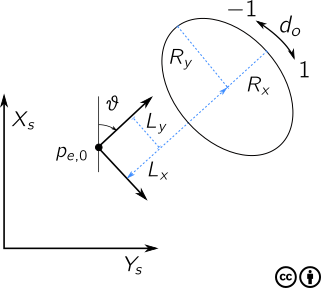
Fig. 7 Ellipse path with translation and rotation.
Straight line
The solution to an initial value problem of a constant velocity particle, such as Eq. (38) is
where \(\theta_l := \col(p_{l,0}, V, \chi)\). Notice that for this parametrization, \(\varpi\) is a time variable in seconds, with \(\varpi = 0\) being the initial condition.
Path-tangential frame and arc length
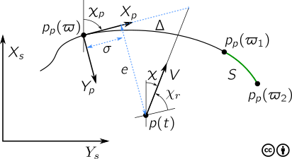
Fig. 8 Path-tangential frame and symbols relating to steering on or to regularly parameterized paths.
In the following, it is useful to confer Fig. 8. The material is taken from [15]. Consider a planar particle \(p_p(\varpi) = \col(x_p(\varpi), y_p(\varpi))\), which is constrained to move along a curve. We define a path-tangential frame as a reference frame with origin \(p_p(\varpi)\) and x-axis aligned with the tangent of the curve. This frame is rotated an angle \(\chi_p(\varpi)\) relative some stationary reference frame using the right-hand screw rule, given by
Consider a particle \(p(t) \in \mathbb{R}^2\), which may change with time \(t\). The error between \(p\) and \(p_p\) can be expressed in the path-tangential frame as
where \(\sigma(t)\) is denoted the along-track error and \(e(t)\) as the cross-track error.
The time rate of change of \(p_p(\varpi)\) is
where we have used the chain rule. The speed of a particle is defined as \(U_p(t) := \|\dat p_p(\varpi)\|\), which also can be written as
The arc length between two points is the distance a particle needs to travel when moving from one point to another. If the particle is constrained to move along a curve, we can show that the time derivative of the arc length is, see e.g. [15]
which confirms that the arc length is the integral of the particle speed. Notice that the arc length increases for increasing parametrization variable \(\varpi\).
Particle feedback laws
We introduce virtual particles, which we can manipulate to achieve various objectives. Usually, the dynamic response of the parametrization variable \(\varpi\) is designed to solve an objective using simple feedback laws. We will cover several such cases in the following.
Particle projection
It is possible to find the point on a curve, which locally minimizes the distance to a point not necessarily located on the curve. The minimization problem
has a local minimum when \(\sigma(t) = 0\). A simple proportional feedback law achieves this:
where \(\gamma > 0\) is the feedback gain. With sufficiently large \(\gamma\), the particle will quickly converge to and be the particle projection of \(p(t)\) as it changes with time.
Path following
The path following algorithm for regularly parameterized paths as described in [8] uses particle projection and lookahead distance to steer a particle \(p(t)\) onto a one-dimensional manifold. We restate the algorithm here, because we will use it in the path planner formulation.
Let \(p(t) \in \mathbb{R}^2\) represent the planar position of a particle in a stationary reference frame. Let \(V(t)\) be the velocity magnitude of the particle, so that
where \(\chi(t)\) is the particle course – the angle between the x-axis and the particle velocity vector.
Define \(p_p(\varpi) \in \mathbb{R}^2\) as a virtual path-constrained particle for which we want \(p(t)\) to converge to an move along. The path following objective is therefore
where we are free to define the dynamics of \(\varpi(t)\). Notice that this objective also can be stated using Eq. (63) as
The dynamics of \(\varpi\) is designed as a combination of particle projection feedback Eq. (68) and a steering law for the orientation of \(p(t)\), given as
where \(\chi_r(e)\) is a path-relative steering angle defined as
with \(\Delta > 0\), see Fig. 8.
The desired orientation of the particle velocity vector is
The control objective of the particle course is to drive \(\lim_{t\to\infty}\chi(t)-\chi_d(e,\varpi) = 0\). The course error is defined as
where \(\tilde \chi\) is to be within the indicated domain, and can be ensured using [8, 15]:
The course rate controller is given as
where \(\omega_{\max}>0\) is maximal rate of turn and \(\Delta_{\dat \chi}>0\) is a rendezvous tuning parameter. This control scheme guarantees that the particle converges to the curve and is proven in [8, 27].
Arc length control objective
Suppose \(p_p(\varpi_1)\) and \(p_p(\varpi_2)\) are path-constrained particles, denoted 1 and 2. Let the control objective be to obtain a desired arc length between the particles, by manipulating the speed of particle 1. Let \(S\) be the desired delta arc length and \(s_{\{1,2\}}\) the arc lengths of the particles. The proportional feedback law for \(s_1\) together with the dynamics for particle parametrizations gives us the following initial value problem
where \(k_d\) is the feedback gain and \(U_{p,2}(t)\) is the speed of particle 2. Note that for \(k_d > 0\), we obtain \(s_1 < s_2\), and vice versa.
Slip angle
We make a clear distinction between course and heading, where course is the planar orientation of the velocity vector in \(\{\text{NED}\}\), whereas heading is the planar orientation of the body frame. We need expressions to relate them to each other and achieve this using geometric relations.
We consider a particle \(p(t) \in \mathbb{R}^2\), which is written in polar form as
where \(V(t)\) and \(\chi(t)\) are the magnitude and orientation of the velocity vector of the particle. Suppose the vector is given as a linear combination of two velocity vectors
where \(\psi\) is heading. Let \(\beta\) denote the slip angle between the heading and course, that is
We can find formulas for \(V(t)\) and \(\chi(t)\), which are expressed in terms of the above variables.
The formula for \(V(t)\) is
We use the geometric relation in Fig. 9 to establish an expression for \(\beta\). It can be seen that \(W\sin(\alpha - \chi) = \ell\), \(U_v\sin(\beta) = \ell\), which gives \(\sin(\beta) = \frac{W}{U_v}\sin(\alpha - \chi)\). The expression for \(\beta(t)\) is thus
When we are given \(\psi(t_0)\), we can calculate \(V(t_0)\) and
With these variables given, we can evaluate \(\beta(t)\) for all \(t\) and also calculate \(\psi(t)\) using the solution to the differential equations of \(\dat p(t), \dat \chi(t)\).

Fig. 9 Geometric relations between two velocity vectors.